A complete agricultural supply model would be defined as a system of equations describing the flow of farm products on to the market. A statistical model is an approximation to the exact relations we put forward in theory, and any single equation we care to consider is an abstraction from the general interdependence of the economic system. The first source of error lies in the aggregate nature of macro-economics. We may expect a reasonable degree of causation between a change in price of a single factor or product and the resulting output, but when output is an aggregate of many different products, each related to its own system of inputs, a certain loss of exactness is inevitable. Second, errors of measurement arise where the yearly definition of variables is made on an arbitrary basis. Farm output and certain seasonal farm inputs, being governed by regular patterns of biological growth, lend themselves to independent yearly observation, but in the case of a price series there may be no clear demarcation between two successive periods of measurement. The use of time series introduces a further error in that the population being sampled may also be subject to change. In particular, it is difficult to allow for the effect of changing techniques over a period of time.
The approximate nature of our equations is recognized by the introduction of a stochastic variable to take care of "unexplainable" variation, whether it arises from inaccurate measurement of a single variable or from the neglect of an important determining variable. The effect of changes in technology can be allowed for by introducing a linear time variable. This implies a constant rate of change only and, as such, may act as a catch-all for all sorts of temporary and permanent influences. On the other hand some form of transformation of the variables may overcome this problem.
The final form of our model is not defined in any precise way, as a number of different lagged values of the independent variables may operate at different times and places. Hence the procedure followed in this article represents a course of trial and error rather than the measurement of fairly rigorously defined postulates. The following section is a brief review of statistical methodology related to single equations, followed by estimates of the supply parameters obtained.
* The latter part of the work involved in this analysis was carried out while the author was supported by a New Zealand University Research Grant. He wishes to acknowledge the considerable help and advice he has received from Dr. H. B. Low, Mr. G. P. Braae, and Professor C. G. F. Simkin.
50
MAY, 1955 |
AGGREGATE SUPPLY OF FARM PRODUCTS |
51 |
If we are to apply tests of significance to parameters estimated by the method of least squares we require the error terms of the regression equation to be random and normally distributed. The presence of a systematic element in the residuals (serial correlation) will mean that the error terms fail to meet the assumption of independence. The problem may sometimes be overcome, however, by the use of first differences of the original values, as suggested by Cochrane and Orcutt.1 Testing the residuals so obtained can be carried out with the Von Neumann ratio,2 or with the distribution prepared by Durbin and Watson3 for a model with the error term randomly distributed.
Further, the presence of more than one independent linear relationship between the determining variables in the regression equation (multicollinearity) may lead to uncertain regression coefficients.4 As we are more interested in the structural relationships than prediction, this consideration is most important. Where the variables are subject to errors of measurement (as is usual) the position is particularly acute, as any regression coefficients obtained will measure partly or wholly the influence of random error terms in the direction in which an actual linear relationship exists.5 They will be further distorted, of course, if vve do not correct for serial correlation. As Stone points out,6 this situation is not necessarily reflected in the standard errors of the regression coefficients. An indication that such a relationship is present is given by unstable or changing partial regression coefficients when a new variable is added. In the following analysis, some general hypotheses are first tested without examining the data for multicollinearity, but the final results are based on an equation selected by means of confluence analysis.
The problem of the errors has already been outlined. Those arising in the process of collection and classification represent the lack of accurate measurement of well-known economic quantities; such errors are increased, of course, when we are forced to rely on substitute criteria. Errors of the equation arise out of the failure to find a complete explanation for the variation of the dependent variable from
1. D. Cochrane and G. H. Orcutt: "Application of Least Squares Regression to Relationships containing Auto-correlated Error Terms", in Journal of the American Statistical Association,, XLIV, 1949, p. 32.
2. J. Von Neumann: "Distribution of the Ratio of the Mean Successive Difference to the Variance", in Annals of Mathematical Statistics, XII, p. 367 (1941).
3. J. Durbin and G. S. Watson: "Testing for Serial Correlation in Least Squares Regression" in Biometrika, XXXVIII, 1951, p. 161.
4. J. Tinbergen: Econometrics, 1951, p. 78.
5. D. Cochrane: "The Measurement of Economic Relationships", in Economic Record, XXV, 1949, p. 7.
6. R. Stone: "The Analysis of Market Demand", in Journal of Royal Statistical Society, CVIII, 1945, p. 297.
52 |
THE ECONOMIC RECORD |
MAY |
its mean. There may be the possibility that an explanatory variable has been neglected, or the lack of complete explanation may be attributed to variables which do not have a constant effect over the period, or to those variables which we know have certain causal relations with the dependent variable but do not yield to statistical measurement.7
The problem of identifying either a demand or a supply relation-ship does not arise as current prices are not related to production in the analysis. All the determining variables are fitted with lags corresponding to the known production period as closely as the data permits with the exception of “current” rainfall.
Apart from statistical requirements, the economic meaning of our data is most closely approximated by the use of a logarithmic transformation. Thus in the equations which follow, the regression coefficients measure elasticities directly, i.e. they indicate the percentage change in output, which will, on average, result from a 1 per cent increase in the input of various factors. The regression model has the general form:
(log X1t - log X1t - 1 = K + b12(log X2t - log X2t - 1) + b13(log X3t - log X3t - 1) + Ut
where
X1t is the dependent variable in period t,
X2t, X3t the independent variables in period t,
X1t - 1, - X2t - 1, X3t - 1 the corresponding values in period t - 1,
b12, b13 the regression coefficients calculated from the the first differences of logs.
K a constant,
and Ut a random error term of zero mean and finite variance.
We may conclude this section with some comments on the selection of variables for the final supply equation. However many relationships we postulate in theory it is almost certain that with such short time series as in general are available, the number of significant relationships in the statistical sense will be somewhat limited. Thus some process of selection is inferred in many cases without any actual statement to that effect. The method used in the present work is the ordinary 5 per cent fiducial limit. A considerable number of different factors which might influence the supply of farm products were thus tested by simple and multiple correlation to determine where the greatest degree of causation appeared to lie.
The final results of this selection process in original logarithms and first differences of logarithms are given in Table 1. The variable
7. These definitions follow Stone, op. cit., 302-3, and Tintner: Econometrics, 1952, pp. 28, 85.
MAY, 1955 |
AGGREGATE SUPPLY OF FARM PRODUCTS |
53 |
X1 denotes the complete New Zealand index for the volume of farm production. “For the compilation of these index numbers,” says the Government Statistician, “a computation has been made for each of the seasons 1928-9 to 1949-50 showing what the annual aggregate value would have been had 1938-9 prices been constant throughout the period. From the resultant aggregates index numbers have been compiled which measure the movements in the volume of production; for since prices were assumed to be constant, volume is the only variable factor in the aggregates.”
X2 is an index of climatic changes. In fact, it represents the total rainfall for the months January, February and March for each year as measured at Ruakura Animal Research Station, near Hamilton, North Island. There are obvious difficulties in obtaining a suitable index for the whole of New Zealand.
X3 denotes the area of hay and ensilage saved by New Zealand farmers in the previous year, t - 1.8
| TABLE I | ||||||
|---|---|---|---|---|---|---|
| New Zealand Farm Supply Equations 1928-50 showing Partial Regression Coefficients, Multiple Determination, and Test for Serial Correlation (See Figure I) | ||||||
| Rainfall | Hay and Silage | R² | “d” | |||
| (1.1a) | .. | .. | 0.1630 | 0.5422 | 0.7765 | 1.020 |
| (1.1b) | .. | .. | 0.4996 | 0.2212 | 0.4662 | 2.295 |
| ±0.1604 | ±0.0761 | |||||
| a. Original logarithm transformation. b. First difference transformation of logarithms. | ||||||
In this investigation first difference transformations are used throughout because it has been found that this method often effectively overcomes the problem of serial correlation and does so here as the table shows.9 The equations show that a considerable proportion of the year-to-year variation in New Zealand farm production can be
8. The volume of farm production series is published annually in the New Zealand Official Year Book. Details of rainfall are published in the New Zealand Gazette. Area cut for hay or silage and area top-dressed every year are found in New Zealand Agricultural and Pastoral Statistics.
9. J. Durbin and G. S. Watson: Op. cit. Having taken first differences we are testing for negative serial correlation in residuals and hence the appropriate test is for the value 4-d which is in this case 1.71. Since the significant upper limit (5 per cent) for twenty-one items and two independent variables is 1.54 we conclude there is no evidence of a significant amount of serial correlation in the residuals. The expected value is 2.10.
10. W. M. Hamilton: “Topdressing and Provision of Winter Feed in Relation to Dairy Production”, in N.Z. Journal of Science and Technology, XXVIA, 1944-5, p. 24.
54 |
THE ECONOMIC RECORD |
MAY |
explained by these two measures of climatic influences. The particular relationship of previous year's crop of hay and ensilage was first isolated by Hamilton10 when considering factors affecting New Zealand dairy production; he attributed the association to the better feeding of cows that would result in the intervening winter. But as the hay and ensilage variable is associated with movements in rainfall in the
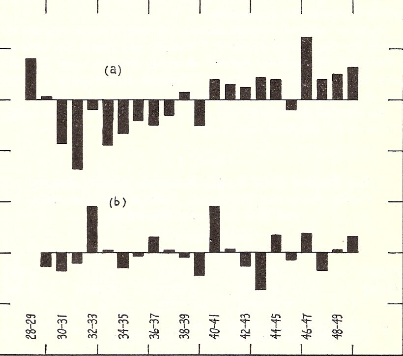
FIGURE I
Distribution of Error Variance from Regression of Climatic Factors on New Zealand Farm
Output. The two distributions are not comparable for individual years.
(a) Logs of original variables, “d” = 1.020.
(b) First differences of logs, “d” = 2.295.
same season (r = 0.57) the feeding factor should be interpreted as a method of transferring the climatic effect from one season to the next. In this particular relation the above transfer effect can be measured with approximately the same accuracy (R² = 0.4492) by substituting a lagged value of rainfall for hay and ensilage in equation (1.1b). In the remainder of the analysis, however, hay and ensilage makes an independent contribution to the explanation of variations in output.
MAY, 1955 |
AGGREGATE SUPPLY OF FARM PRODUCTS |
55 |
| TABLE II | ||||||
|---|---|---|---|---|---|---|
| Partial Regression Coefficients and Multiple Determinations for Regression of Price and Climatic Effects on New Zealand Volume of Farm Production | ||||||
| First differences of Logarithms. N = 21. (1928-50) | ||||||
| Rainfall b12† | Hay and Ensilage b13† | Pricest-1 b14 | Pricest-2 b15 | Area T.-Dressed b16 | R² | |
| (1.2) | 0.5007 | 0.2231 | 0.0078 (0.0744) | 0.4706 | ||
| (1.2a) | 0.4933 | 0.2478 | 0.0998 (0.0783) | 0.5128 | ||
| (1.3) | 0.4959 | 0.2049 | -0.741 (0.0941) | 0.4976 | ||
| (1.3a) | 0.4935 | 0.2135 | -0.1251 | 0.5463 | ||
| (1.4) | 0.4365 | 0.2081 | -0.0478 (0.0901) | 0.1212 (0.1041) | 0.5032 | |
| (1.4a) | 0.4768 | 0.2427 | 0.0818 (0.0831) | 0.0376 (0.0940) | 0.5165 | |
| (1.5) | 0.4329 | 0.1963 | -0.1081 (0.0858) | 0.1310 (0.0919) | 0.5541 | |
| (1.5a) | 0.4284 | 0.2104 | -0.1554* (0.0714) | 0.1359 (0.0844) | 0.6097 | |
| (1.6) | 0.4209 | 0.1900 | -0.0279 (0.0891) | -0.1041 (0.0771) | 0.1490 (0.1108) | 0.5570 |
| (1.6a) | 0.4487 | 0.2365 | 0.0972 (0.0856) | -0.1618* (0.0711) | 0.0786 (0.0977) | 0.6406 |
We can now introduce the economic question of whether, having corrected approximately for climatic influences, we can isolate a systematic price element in the production series. Five equations are presented in Table II; each being estimated with deflated prices as well as with actual prices. A further variable, area of pasture top-dressed with superphosphate and/or lime for the whole of New Zealand, is also introduced.11
11. Over the period 1928-50 the correlation of first differences between nominal export prices in period t-1 and top-dressing in period twas 0·53, and that of the deflated series with the same lag was 0·52. In the period t-2 the corresponding figures were 0·31 and 0·25 respectively. Owing to these relationships the top-dressing variable in the equations is non-significant.
56 |
THE ECONOMIC RECORD |
MAY |
X4 is Export Prices in the year ended 30th June t - 1.
X5 is Export Prices in the year ended 30th June t - 2.
X6 is the area top-dressed in the January year, t- (5/12)
As might be expected from the coefficients of determination in Table I, the use of the first difference transformation in Table II has resulted in fairly large errors of the equation in each case. This is partly explained by the lack of suitable variables besides those considered, but must largely be attributed to the use of the first difference transformation with a variable, namely, rainfall, which is particularly subject to errors of measurement.
The addition of one or other of the price variables by itself appears to add very little to the variance explained in equation (1.1b). The deflated series might be said to be the more significant of the two, but at such low levels of significance that a conclusion is exceedingly tentative. This result is corroborated, however, by the improvement in the explanation when top-dressing is introduced.11 The two-year response also shows out more clearly. It will be noted that the deflated b15 is significant at the 5 per cent level in equations (1.5a) and (1.6a) while b14 and b>16 are not. Such a relationship is rather suspect from the statistical point of view, for with successive manipulations of such a short series, we can expect sooner or later a significant relation at the 5 per cent level to turn up purely by chance. There is also the problem of multicollinearity to be taken into account. We propose to deal with it below.
Our preliminary conclusion, at this stage, is that we have failed to isolate any real price influences in the farm production series. We have only a negative indication that the supply function of New Zealand agriculture is highly inelastic. In other words, not only is the supply of farm products independent of the current market situation, but it also tends to be independent even of previous market situations.
To measure more accurately the effect of the seasonal variables used, especially X2, Ruakura rainfall, the field of investigation was narrowed down to the Waikato area itself. This area is predominantly dairying, so that the dependent variable “butterfat supplied to factories”12 may be expected to be directly related to climatic variations. Data for the other independent variable, crop of hay and ensilage
12. This information was specially extracted from the records of the Census and Statistics Department, Wellington. The author wishes to thank the Government Statistician (Mr. G. E. Wood) for allowing him access to these confidential records. A certain error exists in the data as the factory returns are collected for the year ending March 31.
MAY, 1955 |
AGGREGATE SUPPLY OF FARM PRODUCTS |
57 |
saved, also relate to this area.13 It was possible in this case to extend the analysis to cover the thirty-three years from 1918 to 1951.
The variables are, finally:
X1 = Butterfat supplied to Waikato factories,
X2 = Ruakura rainfall,
X3 = Hay and ensilage saved in Waikato from the previous season,
X4 = Factory payout during the previous season.14
Two equations in first differences of logarithms follow:
| (3.1) | X1 = K + | 1.4068 (0.2748) | X2 + | 0.3818 (0.0951) | X3 | R² = 0.6537 | |
| (3.2) | X1 = K + | 1.2855 | X2 + | 0.3753 | X3 | + 0.1011 X4; | R² = 0.6619 |
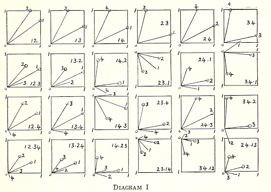
DIAGRAM I
Normalized Regression Slopes, Waikato Supply Function, 1918-52
The marked effect of variations in summer rainfall on dairy production in the Waikato is clearly brought out. Since one-third of the total cows in milk in New Zealand are in this area, the variation in
13. The hay and ensilage and top-dressing data were extracted from the agricultural and pastoral statistics for the region which was thought to supply butterfat to the factories selected in (12) and which also had some climatic kinship with Ruakura. The counties covered are Manakau, Franklin, Raglan, Waikato, Thames, Hauraki, Ohinemuri, Matamata, Piako, Waipa and Otorohanga.
14. Average payout by dairy companies for butterfat for butter.N.Z. Dairy Board Report, 1948-9, p. 8.
58 |
THE ECONOMIC RECORD |
MAY |
summer rainfall at Ruakura will have a reasonably strong influence on total butterfat for New Zealand, and even on aggregate farm output.
The normalized regression slopes are set out in Diagram 1. The set (123) is given in equation (3.1). The addition of price in (1234) (equation 3.2) indicates that the resulting equation is multicollinear. We are not in a position therefore to use any price elasticity so obtained for policy purposes, as it must necessarily be influenced by the presence of an “unexpected relationship”.
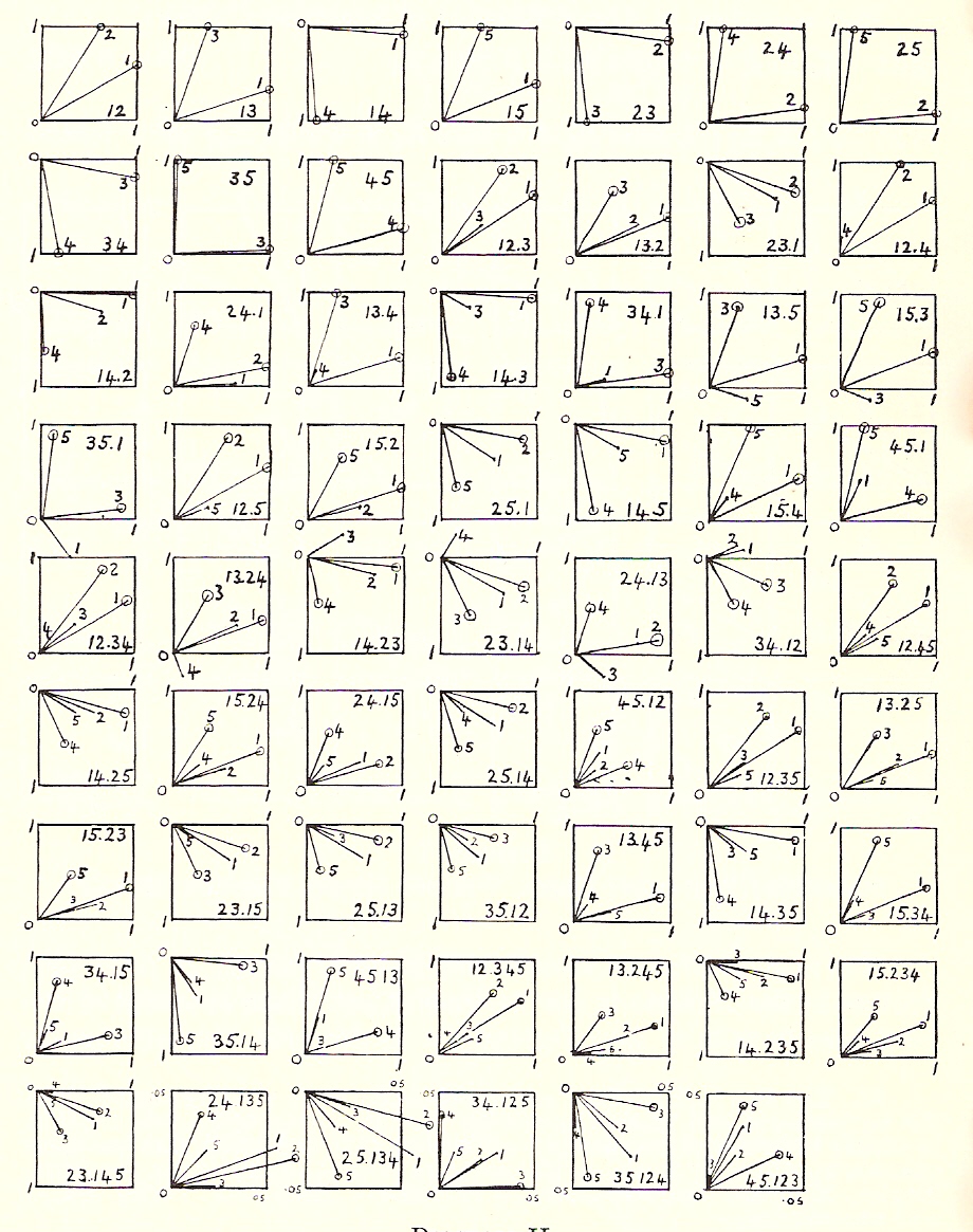
DIAGRAM II
Normalized Regression Slopes, Waikato Supply Function, 1926-52
MAY, 1955 |
AGGREGATE SUPPLY OF FARM PRODUCTS |
59 |
Since top-dressing data has only been collected from 1926, the rest of this analysis is restricted to the 26-year period 1926-52. Diagram II sets out the results of the confluence analysis. The subscripts 1, 2, 3, 4, remain the same as in the 33-year analysis, top-dressing being designated X5 in this case. The number of different price situations has been narrowed down to the single relationship which looked most promising so as to keep the computations within reasonable bounds. Possible equations are presented in Table III.
| TABLE III | ||||||
| Waikato Regression Coefficients and Multiple Determinations,1926-52 | ||||||
| Rainfall b12 |
Hay and Silage b13 |
Price (t - 1) b14 |
Top- dressing b15 |
R² | ||
| (3.3) | . . | 1.2364 (0.2877) |
0.2750 (0.1053) |
0.5082 | ||
| (3.4) | . . | 1.1640 (0.2652) |
0.2633 (0.0966) |
0.3740 (0.1625) |
0.6073 | |
| (3.5) | . . | 1.2053 | 0.2351 | -0.1828 (0.1185) |
0.6490 | |
| (3.6) | . . | 1.2659 | 0.2697 | -0.1000 (0.1304) |
0.5216 | |
| (3.7) | . . | 0.1872 | -0.1256 (0.1662) |
0.5052 | 0.2679 | |
| (3.8) | . . | 1.1366 | -0.2387 (0.1334) |
0.4792 | 0.5424 | |
From Diagram II, however, we see that not all of the above equations are acceptable owing to a suspicion of multicollinearity. The only consistent three-set is (123) and as the higher sets are not satisfactory we are forced back to the same group of variables in equation 1.1b of Table I.
This last result indicates that yearly variations in the supply of butterfat are more related to climatic changes than to changes in price the preceding year. Although the Waikato basin is not entirely given over to dairy production (the ratio of milking cows to sheep is 1: 2 - 9) the lack of price responses suggests that butterfat output tends to behave like an aggregate itself, rather than as a price-sensitive component of the national aggregate. The reason for this lies, of course, in the immense natural advantages that this grassland dairying pattern has over other possible alternatives at present-day prices.
60 |
THE ECONOMIC RECORD |
MAY |
In general the failure to isolate some chain of causation between changes in price and subsequent changes in output supports the hypothesis that dairy output can be regarded as an autonomous variable in any future New Zealand studies in econometrics. Clearly some other types of farm production than dairying may still remain exceedingly sensitive to market changes and in such cases could not be regarded as wholly predetermined.
The low values obtained for the partial regression coefficients of price on production at least indicate that the one-year supply curve of agriculture is nearly vertical and that in some periods of years it leans somewhat to the left and in others somewhat to the right. The positive slope of dairy output for 1919-52 is a reflection of rapid development in the early 'twenties when, by and large, prices were also favourable. The negative slope for 1926-52 is a reflection, on the other hand, of the depression when marked climatic rises in butterfat production were associated with unfavourable movements in prices. Since 1940, the slope has undoubtedly moved over to the right again. These conclusions fit quite satisfactorily into some of the recently published work of W. W. Cochrane in the U.S.A.15
The mechanism by which farmers adjust production requires some comment. Changes in price may have two effects which, in a single product type of farm such as a dairy farm, tend to counteract one another. Higher prices may tend to increase marginal inputs in accordance with marginal productivity theory but, at the same time, the higher income reduces pressure upon the farmer and probably causes him to take some of his increased real income in the form of leisure.
Finally the period of years selected must influence the resulting regression. Since 1918 there have been so many and so marked technological and economic changes in the population we have been measuring that any assumption of a homogeneous or stable economic structure is almost certainly wrong. These considerations point to the analysis of a reasonably short period of time, certainly much shorter than that strictly required for a time series analysis. In the long run increases in farm output are dependent on the direct adoption of new techniques whatever the particular stimulus for such changes happens to be.
R. W. M. JOHNSON
Massey Agricultural College.
15. W. W. Cochrane: "An Analysis of Farm Price Behaviour", in Pennsylvania State College, Progress Report, No. 50.