by
Rod Forbes and Robin Johnson2
These estimates of Tornqvist productivity indices were first prepared for a productivity conference at the University of New England in 1995 (Johnson 1996). That paper compared Tornqvist indices with Laspeyre (base-weighted) type volume indices, and discussed the reasons for using geometrically weighted factor shares as weights. The present paper updates the data series from 1992 to 1998 and checks out the earlier results and their implications.
Tornqvist weighting can be used for a total input productivity index (TIP) or a total factor productivity index (TFP). The total input index takes account of changes in the composition of intermediate inputs as well as labour and capital inputs. The total factor productivity index simply expresses net real output as a function of labour and capital input. In national accounting terms, intermediate inputs are deducted from gross output to obtain factor or net output for an industry. Using national accounting conventions involves important assumptions about the marginal returns to intermediate inputs.
Tornqvist weighting is used to overcome biases caused by changes in the respective weights of the components of a given volume index. In the case of intermediate inputs, for example, the use of fertiliser may be changing systematically during the period of observation. Base year weights of different inputs would freeze the true weighting over a period of time. Similarly for the total fertiliser index of volume - a base year weight would freeze the mix of different fertilisers when farmers were changing their respective mixes. These biases can thus arise from any change of use in a productive input and are commonly found in fertilisers, weedkillers, sprays, and other inputs. The same reasoning applies to changes in the mix of outputs.
In the agricultural sector, national accounts on an SNA basis are available back to the 1950s. The accounts present nominal estimates of gross output, intermediate inputs and net income (equivalent to gross domestic product). For productivity analysis, these entities must be converted to volume terms. In the case of the agricultural sector, real inputs are deducted from real gross output to obtain real net output. Both gross output and intermediate inputs are deflated separately. Estimating these volume series may be by one implicit index or by the use of price indices for each component of gross output and intermediate inputs. In turn these price series are derived by statisticians from surveys of the productive sectors. In doing so, the statisticians adopt various methods to weight the individual components of a price index. A base year weighting system introduces the same biases as for the input volume series. Theoretically, such price indices should also be geometrically weighted as well. This would involve complete access to the data bases of the statisticians if it were to be carried out systematically.
The present paper sets out the methodology of estimation of Tornqvist indices of agricultural productivity for New Zealand since 1972, and then examines the impact of different weighting systems on estimates of TIP and TFP. The use of service costs of capital are discussed and compared with factor shares based on the national accounts. Different methods of depreciating capital stocks are discussed and the results compared. The overall results are compared with other sectors of the economy for which comparable data is available.
The national income identity for nominal factor income is as follows:
(1) FI = PQ - SM
FI = factor income (GDP)
PQ = value of gross output (P = price)
SM = value of intermediate inputs (S = price).
The underlying profit maximisation equation can be written:
(2) pi = PQ - SM - WL - RK
WL = reward to labour (W = price)
RK = reward to capital (R = price)
In real terms, factor income (FI*) is estimated by the double deflation method:
(3) FI* = PQ/P - SM/S
Since the aggregates are composed of the individual input (i) and output (j) categories, (3) can be written as:
(4) FI*t = Ej Pjt Q jt / Pjt - E i S it Mit / Sit
where Pjt Qjt = price and quantity of the jth output category in year t,
and Sit M it = price and quantity of the i thinput category in year t.
The factor income productivity index can be defined as:
(5) FIPt = ( FI*t / W o L t + R o K t )
This can be rewritten to include base year prices for factor income:
(6) FIP t = ( Po Q t - S o M t / W o L t + R o K t )
where P o , S o , W o, R o , are the prices of the base year.
A total input productivity index may also be defined in the same way:
(7) TIPt = ( Po Qt / Wo Lt + Ro Kt + So Mt ).
To overcome the base year bias problem in the volume indices and the price indices, the Tornqvist discrete approximation to a Divisia Index is used here. This defines the Index, Q t , as the weighted change in the proportions of its base weighted value components:
(8) Q t = pi t ( Q it / Q io ) 1/2 (w it + wio )
This can be transformed by logarithms to the base e to give the estimation formula:
(9) ln Qt = Ei 1/2 ( w it + w io ) ( ln Q it - ln Q io )
where wit = the share of the i th input (j th output) in total nominal input
(output) in the year t, and
w io = the share of the i th input (j th output) in total nominal input
(output) in the base year.
The Tornqvist Index estimates the rate of change in aggregate inputs or outputs from the geometrically weighted rate of change of the components of total input and total output. Average percentage growth rates can be estimated from this index. By taking anti-logs, the base year takes on a value of 1.000.
In most studies of factor productivity, factor income is derived from the national accounting identities and then expressed as a ratio of factor income to the weighted average input of labour and capital (equation 6). In this study, the accounting identity for intermediate inputs is not utilised and the Divisia weighted volume index is substituted. Thus we have an expression for factor income which is derived from two Divisia weighted aggregates (total output and total inputs) which is then compared with a Divisia weighted average of capital and labour inputs. Alternatively, the total input factor productivity ratio can be estimated by comparing Divisia weighted total output and the Divisia weighted average of labour, capital and intermediate inputs.
e.g. Divisia factor income = Divisia total volume index - Divisia intermediate inputs
Divisia factor productivity = Divisia factor income/ Divisia combined factor inputs.
Since two indices cannot be subtracted, the equivalent value series is derived for each series , subtracted, and then converted back to an index.
The weighting of capital and labour inputs should follow, in theory, the procedure devised by Tornqvist. That involves determining the nominal shares of factor income going to labour and capital (including depreciation). Most national accounts divide factor income into rewards to labour, consumption of capital, interest paid and operating surplus plus a correction for subsidies and taxes. One method is to accept the wage component as a "paid" reward and attribute the remainder of factor income to capital reward. This gives a nominal factor share that does not vary much from year to year.
Another method is to estimate capital rewards first and make wage rewards the residual. This procedure was followed in the previous paper (Johnson 1996). In that paper, depreciation of capital was estimated from the annual wastage of capital assets, and the service cost of capital. This is a debt-equity approach to the relevant factor shares. The service cost of borrowed capital (SC) is estimated as follows:
(10) SC t = A t (( d t / 100 ) + ((1-e t ) (m t / 100 ) (n t / m t )))
where A t = nominal asset value at beginning of year t,
d t = wastage or disappearance rate in during year t,
e t = equity to asset ratio in year t,
m t = interest rate on new mortgages registered in year t,
n t = actual average interest rate paid on sheep farms in year t.
In general, wastage rates are slightly higher than conventional depreciation rates, while the service cost of capital is lower than the full opportunity cost of capital including equity. The factor share of labour varies considerably by this method over a period of time. The resulting factor shares in total factor income are shown in Figure 1.
Remember the objective is to determine appropriate weights in nominal terms for the application of the Tornqvist formula. By using service cost of capital as the weight for capital input volumes, the balance of net output must be considered the labour share made up from equity returns on capital and paid wages3. This recognises the special position of self-employed entrepeneurs (i.e. the farmers).
The definition of the capital stock variable requires further discussion. The previous study employed a device to estimate wastage of capital directly. This was possible because of the special attributes of the agricultural sector data where comparisions could be made of the “disappearance” of capital over a specified period of time. Philpott (1995, 1999a) provides another series of capital stocks derived from business depreciation rates. This results in a series not dissimilar to the wastage series. Allternatively, Philpott (1994, 1999a) provides estimates of capital stock based on a vintage model where “disappearance” is estimated for whole blocks of assets on a systematic basis. Philpott's gross capital stocks tend to be 50 per cent higher than his net capital stocks. The gross series is used in this study for measuring real assets employed. All capital stocks are derived from a perpetual inventory model in terms of the following identity:
(11) Kt = (1 - f) K t-1 + E t-1
where K t = the stock of conventional capital at the beginning of period t in constant prices;
K t-1 = the stock of capital at the beginning of period t- 1;
E t-1 = capital expenditure during period t- 1 in constant prices; and
f = the depreciation or obsolescence rate of capital chosen.
For a discussion of the choice of starting dates see Philpott (1994), Industry Commission (1995), Diewert and Lawrence (1999), Philpott (1999b) and Johnson (1999).
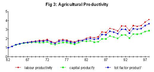
The volume of real net output (real factor income) has increased steadily over the period from1972 to 1998 with little growth in total labour employed and real gross capital stock employed (Figure 2). The labour force has been in decline since 1982 and the capital stock employed has been in decline since 1987. The average rates of growth on an annual basis are shown in Table 1.
| Table 1: Main TFP parameters | |
|---|---|
| (base year weights) | |
| (trend % per annum) | |
| Labour force | -0.3 |
| Capital stocks | -0.1 |
| Real factor income | 4.0 |
| Labour productivity | 4.3 |
| Capital productivity | 4.0 |
| Total factor productivity | 4.1 |
Figure 2 shows the trends in labour and capital productivity and the weighted mean of the two. Fluctuations in productivity are caused by changes in national income from agriculture rather than from the input series. The average rate of change is shown in Table 1.
The rates of change shown in Table 1 are derived from regression estimates of the rate of change over the whole period. Table 2 shows the goodness of fit statistics for the regressions for the variables entering into the total productivity and the factor productivity estimates. Where the Durbin-Watson test was poor, a first difference transformation was explored. The different specification does not change the growth rate estimates by a great margin.
| Table 2: Goodness of Fit for Whole Period 1972-98 | ||||||
|---|---|---|---|---|---|---|
| Original data | First differences | |||||
| Tornqvist | b | R2 | DW | b | R2 | DW |
| output | 1.6 | 0.90 | 1.41 | 1.6 | 0.91 | 2.01 |
| all inputs | 0.7 | 0.02 | 1.54 | - | ||
| TIP | 1.5 | 0.86 | 1.27 | 1.6 | 0.85 | 2.16 |
| factor income | 3.4 | 0.88 | 1.86 | - | ||
| factor inputs | -0.2 | 0.12 | 0.24 | -0.6 | 0.24 | 2.33 |
| TFP | 3.5 | 0.87 | 1.52 | - | ||
| Laspeyre | b | R2 | DW | b | R2 | DW |
| output | 1.8 | 0.92 | 1.15 | 1.9 | 0.87 | 2.04 |
| all inputs | 0.9 | 0.03 | 1.67 | - | ||
| TIP | 1.7 | 0.89 | 1.15 | 1.8 | 0.86 | 2.06 |
| factor income | 4.0 | 0.91 | 1.66 | - | ||
| factor inputs | -0.1 | 0.05 | 0.21 | -0.5 | 0.23 | 2.37 |
| TFP | 4.1 | 0.89 | 1.38 | 4.4 | 0.90 | 1.99 |
Table 3 shows total input productivity (TIP) estimated by base-weighted methods (Laspeyre indices) and by Tornqvist geometric weighted methods. The latter weights are derived from average value shares between the current year nominal factor shares and the base year factor shares. If an input or an output mix is changing in a systematic way the geometric method makes the appropriate adjustment. Figure 4 shows a comparision of the of the two weighting methods for gross output of the agricultural sector; Figure 5 shows the comparision for total inputs employed; and table 6 shows the comparision for the total input productivity index (TIP).
| Table 3: Total Input Productivity by Weighting Method and Periods (growth rates) | ||||||
|---|---|---|---|---|---|---|
| Tornqvist | Laspeyre | |||||
| Output | Input | TIP | Output | Input | TIP | |
| 1972-84 | 1.1 | 0.5 | 0.6 | 1.0 | 0.3 | 0.7 |
| 1985-98 | 1.8 | 0.0 | 1.8 | 2.2 | 0.3 | 1.9 |
| 1972-98 | 1.6 | 0.7 | 1.5 | 1.8 | 0.9 | 1.7 |
Total input productivity tends to be over-stated by base-weighted indices particularly since 1985. Thus the better estimate of long run total productivity is 1.5% per year since 1972. Both methods suggest that the rate of growth has improved since 1985 compared with the earlier period 1972-84. Table 4 shows the same results for total factor productivity and Figure 7 shows a comparision of the two weighting methods for the TFP ratio.
| Table 4: Total Factor Productivity by Periods (growth rates) | ||||||
|---|---|---|---|---|---|---|
| Tornqvist | Laspeyre | |||||
| Income | Input1 | TFP | Income | Input | TFP | |
| 1972-84 | 2.6 | 0.8 | 1.8 | 3.1 | 0.9 | 2.2 |
| 1985-98 | 3.2 | -0.8 | 3.7 | -0.6 | 4.3 | |
| 1972-98 | 3.4 | -0.2 | 3.5 | 4.0 | -0.1 | 4.1 |
| 1Total factor input | ||||||
Again Tornqvist indices tend to lower the factor income increase and the factor input increase (slightly) with the resulting effect on the productivity growth rate. Thus the best estimate for factor productivity growth for the period since 1972 is more likely 3.5% per year rather than 4.1% per year as might have been indicated by base weighted indices.
Diewert and Lawrence estimate the rate of growth of factor productivity in agriculture for the period 1978 to 1998 as 3.87% per year. This lies between the above two estimates. For more careful comparision we need to look at the specification of their model.
“To form separate TFP indexes for the 20 industries we now take real production GDP as output, normalise it to equal 1 in 1978, and form a chained Fisher index of the three industry inputs - labbour hours, plant and eqipment stocks, and building and construction stocks - using labour costs and capital user costs as weights. We then take the ratio of the industry's total output to total input indexes to form the industry's TFP index. The industry TFP indexes use our ptreferred base case specification of production base GDP, the database's composite labour series, and our net capital estimates”.
The chained Fisher index gives very similar results to the Tornqvist index - it being the geometric average of the Paasche and Laspeyre indexes. Production based GDP is the same as used above; the use of labour hours tends to increase the input of labour and decrease the resulting TFP; and the net capital stock grows more slowly than the gross capital stock used above. Thus the Diewert and Lawrence results are lower by reason of their labour definition but higher by reason of their capital definition. A summary of their sector estimates of industry TFP growth by their methodology is shown in Table 5.
| Table 5: TFP's by Diewert and Lawrence (1978-98) | |||
|---|---|---|---|
| Agriculture | 3.87 | Fishing | 0.25 |
| Forestry | 6.34 | Mining | 4.92 |
| Energy | 3.50 | Construction | 0.63 |
| Trade, Rest'rants | -0.75 | Transport | 3.87 |
| Communications | 6.77 | Finance services | -2.11 |
| Community services | 0.03 | Textiles | 0.68 |
| Wood products | 0.30 | Food & beverages | 0.68 |
| Paper products | 1.28 | Chemicals | 0.25 |
| Non-metallic min | 2.36 | Basic metals | 1.01 |
| Machinery | 0.03 | Other manuf'ing | 2.43 |
The particular reasons for the growth or lack of growth in each sector needs to be examined against the background of labour and capital input changes, the uptake of technology, and other factors which might bear on productivity increases. This data does give a uniform set of answers though as Diewert and Lawence point out there are still definitional problems in some sectors (particularly the service sectors) which need to be resolved. For the record, the agriculture sector is third equal in the productivity comparisions over the period concerned.
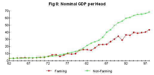
Agricultural producers in New Zealand continue to complain of the low incomes they receive (compared with the past). Clearly, the high gains in productivity have not been translated into farm incomes. This can be seen from a comparison of nominal GDP earned in farming compared with the rest of the economy (Figure 8). Up to 1978, farm producers earned comparable incomes in GDP terms to the rest of the economy. Since that time, there has been a consistent deterioration in relative incomes. How has this come about?
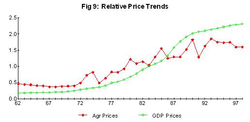
The main determinant of changes in farming incomes is the terms of trade. This is shown by a comparison of the price deflators for farming and national income (Fig 9). Farmers are at the mercy of international commodity price trends, modified by changes in the exchange rate, and these trends have lagged well behind average prices in New Zealand since 1962.
It has to be concluded that farmers have to keep running to stand still. Without productivity increases their incomes would be unacceptable. Resources would have moved out of farming and exports of tradeable goods would have declined. The NZ economy would have slumped and the welfare burden would have become unacceptable. Presumably, some sort of equilibrium would have been restored by adjustments in the exchange rate with consequent implications for the price of imported capital and consumer goods.
Diewert, E., and Lawrence D. (1999), Measuring New Zealand's Productivity, Working Paper prepared for NZ Treasury, (http://www.treasury.govt.nz/working papers).
Industry Commission (1995), Research and Development, Vols I - III, AGPS, Canberra.
Johnson, R.W.M. (1996), Agricultural Productivity Trends for New Zealand 1972-1992, MAFPolicy Technical Paper 96/2, Ministry of Agriculture, Wellington.
Johnson, R.W.M. (1999), The Rate of Return to New Zealand Research and Development, Paper presented to the NZ Association of Economists, Rotorua, July.
Philpott B.P. (1994), Data base of Nominal and Real Output, Labour, and Capital Employed by SNA Industry group 1960-1990, RPEP Paper 265, Victoria University, Wellington N.Z.
Philpott B.P. (1995), Real Net Capital Stock by SNA Production Groups New Zealand 1950-1991, RPEP Paper 270.
Philpott B.P. (1999a), Provisional Estimates for 1990-1998 of Output, Labour and Capital Employed by SNA Industry Group, RPEP Paper 293.
Philpott, B.P. (1999b), Deficiencies in the Diewert-Lawrence Capital Stock Estimates, RPEP Paper 294.
[1] Contributed paper to the Annual Conference of the Australian Agricultural and Resource Economics Society, Sydney, January 23-25, 2000.
[2] Ministry of Agriculture and Private Consultant respectively.
[3] The national income identity is W+D+OS+IT-S. Paid interest is deducted from operating surplus. Thus if capital shares are based on depreciation and debt servicing, the wage share is the balance of operating surplus adjusted for indirect taxes and subsidies and wages paid.
[4] The necessary details for re-weighting the national set of national income data is only available back to 1972, and then with some extrapolation. Some of the illustrative figures in the paper are derived from non-weighted data back to 1962.